In this post I will present two model economies that should be useful for anyone who wants to get into planning. The economies are formulated as linear programs, and the goal is to find optimal solutions to these programs. I will also provide a sketch for an interior point algorithm, mostly lifted from existing literature. Finally I have a few words on how to solve LPs of this type in a distributed manner.

The models

The model economies presented here exploit a few notions:

• in real economies, firms only depend on a finite set of other firms much smaller than the economy as a whole
• the average number of firms any one firm depends on is bounded by some constant $q$ regardless of the size of the economy
• the economy has a small set of core industries and a larger "long tail" of less crucial industries
• core industries have lots of industries that depend on them, whereas the rest do not

There are three components to the models:

• technical coefficients
• a number of extra "basket" constraints
• balance equations to enable optimization

The difference between the models is the structure of the technical coefficient matrices. Five parameters determine the size and density of the resulting system matrix $S$:

• $v$ the number of industries
• $q$ the number of inputs to each industry, as described earlier
• $w$ the number of basket constraints
• $r$ the density of each basket constraint
• $o$ the number of balance equations to optimize over

The technical coefficients are of the same sort as those used by Leontief. They are arranged so that columns contain the inputs of each firm, and rows correspond to outputs. The diagonal is the identity matrix. Off-diagonal elements are negative. The coefficient matrix must satisfy the Hawkins–Simon (HS) condition. Both matrices are generated through a preferential attachment process, and the process used is the difference between the two models. More on that later.

The right-hand side for the technical coefficients are a given list of demands. Leontief's formulation $(I-A)x=d$ is relaxed to $(I-A)x\ge d$.

The "baskets" are an additional set of constraints. They allow having multiple technologies available for producing a single good, or a class of goods. They take the form $Bx\ge f$, where both $B$ and $f$ are non-negative. We can imagine any number of these extra constraints. A concrete example would be the nutrition constraints in the last post.

The name "basket" comes from something I read about how Gosplan worked. Due to limited computational resources Gosplan could not plan things using disaggregated data. Instead they had to group goods into into so-called baskets of goods, and issue aggregate plan targets. This is frankly a very shitty way of planning things, and it should not be construed that I am in favor of the ad-hoc planning system used in the USSR. I am merely borrowing the terminology. There are more ways in which Gosplan failed to produce rational plans, but such criticism I leave for a potential future post.

The purpose of adding extra constraints like this is so that we can evaluate what happens if we decide to relax some set of demands (entries in $d$) to free up resources for other things. The baskets then act as a set of "sanity checks" so that there is no catastrophic shortfall in essential goods. In other words $d$ can be viewed as a set of wants while $f$ is a set of needs. In liberal economics, wants and needs are considered demands of equal importance, but the scheme presented here gives us more "wiggle room". Another use for these contraints is to be able to say "produce at least this many MWh of electricity", not caring particularly how that electricity is produced. Then one can check what happens if coal fired power plants are successively shut down and replaced by nuclear and renewable power.

Finally there is a set of balance equations meant for the optimization to work on. This can be things like labour time spent, CO2 released, capital stocks consumed and so on. The balance equations can be sparse, but in these experiments I have chosen to make them dense.

For the balance equations the right-hand side is all zeroes. Using non-zero values is possible, but they are easily subtracted away due to the presence of the identity matrix. Using zeroes increases the sparsity of the system and hence makes a solution easier to compute.

Finally, all variables must be positive.

In summary the system looks like this:

$Sx=\left[\begin{array}{cc}I-A& 0\\ B& 0\\ -O& I\end{array}\right]x\ge \left[\begin{array}{c}d\\ f\\ 0\end{array}\right]=b$

$A\in {\mathbb{R}}^{v\times v},B\in {\mathbb{R}}^{w\times v},O\in {\mathbb{R}}^{o\times v}$

$S\in {\mathbb{R}}^{(v+w+o)\times (v+o)}$

The goal of the solver is to find the optimal solution $x_{*}$ defined as follows:

$x_{*}=\underset{\begin{array}{c}Sx\ge b\\ x\ge 0\end{array}}{\arg \min }\sum _{i=v+1}^{v+o}{x}_i=\underset{\begin{array}{c}Sx\ge b\\ x\ge 0\end{array}}{\arg \min }{c}^{T}x$

­$c$ is a vector of $v$ zeroes followed by $o$ ones.

The structure described above makes computing an initial strictly feasible solution straightforward:

$x_v=(I-A{)}^{-1}d$

$u=\underset{i}{\max }\frac{f_i}{B_i{x}_v}$

$x_o=O{x}_v$

$x_{(0)}=1.1\left[\begin{array}{c}u{x}_v\\ x_o\end{array}\right]$

In other words, first a Leontief solution $x_v$ is computed for the coefficient matrix. Then a value $u$ is computed which makes $u{x}_v$ satisfy the basket constraints. Then $x_o$ is computed so that the balance equations are satisfied. The final $x_{(0)}$ is assembled from $x_v$, $x_o$ and $u$ and scaled up by 10% so that it forms a solution that is strictly inside the feasible set.

On to the technical coefficients:

Price's model

Since industries pop up over time it seems reasonable to pick a model that is designed to produce power-law distributed graphs. One such model is Price's model, named after Derek J. de Solla Price. This model is intended to model citation networks, which grow over time. More famous papers tend to be cited more often, and the citations form a directed acyclic graph (DAG). Price's model results in that the distributions of citations follows a power law.

One drawback of Price's model as applied to economics is that real world economies do not look like a DAG. Recycling especially breaks Price's model. Nevertheless this model is useful because the distribution of row and column ranks is known. Since the resulting incidence matrix is triangular, computing $x_v$ is especially easy for this model, requiring only $O(\mathrm{nnz}(A))$ operations.

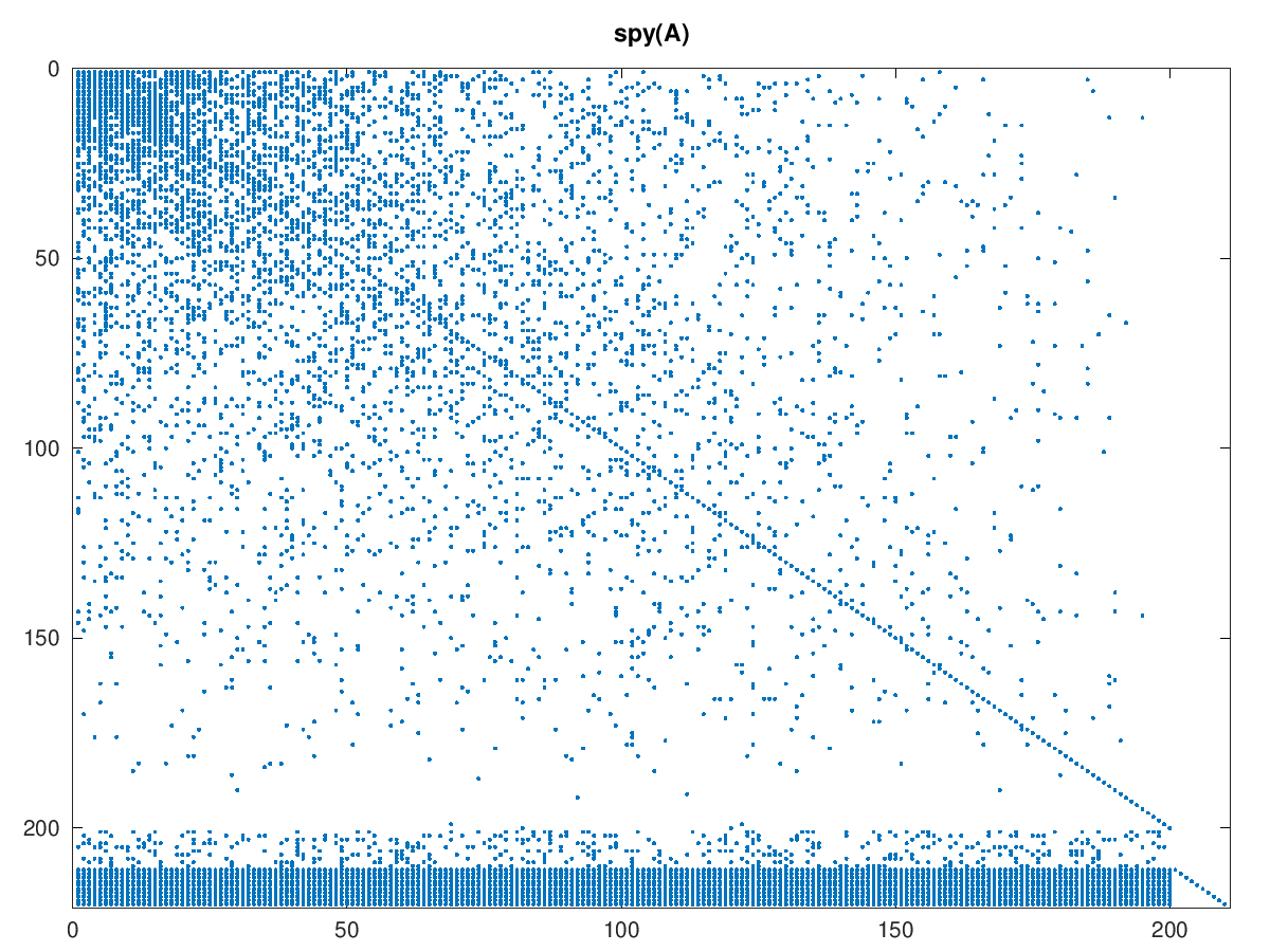
The sparsity pattern of the Price model looks like this:

The triangular structure is apparent, as are the coefficients for the baskets and balance equations. To me this model seems to result in an overemphasis of very few core industries. It is also naïve in that it assumes old established industries do not make use of new technology. This is also not the model I started my experiments with.

Interdependent model

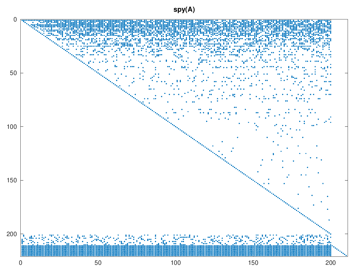
The initial model used in my experiments is one where industries grow interdependent over time. It differs from Price's model in that after each new node added, $q$ new links are made equiprobably between any pair of nodes added so far. This produces a matrix where non-zeroes are clustered in the upper left corner, growing more sparse toward the right and the bottom:

Here the economy is quite explicitly not a DAG. Computing $x_v$ is also more expensive, but still quite cheap using iterative methods. We could also choose to compute the inverse of the upper left block of core industries explicitly, which would be useful as a preconditioner.

Optimality and the duality gap

When we're optimizing it is useful to know whether we are close enough to the optimal solution. We'd like some sense of how much "room" there is for further optimization, preferably some lower bound. If we know that we are within say 1% of this lower bound then we can stop. Such lower bounds are given by feasible solutions to the dual of our starting program.

Instead of seeking the minimal solution to the primal:

$x_{*}=\underset{\begin{array}{c}Sx\ge b\\ x\ge 0\end{array}}{\arg \min }{c}^{T}x$

we instead seek to maximize its dual:

${\lambda }_{*}=\underset{\begin{array}{c}{\lambda }^{T}S\le c^T\\ \lambda \ge 0\end{array}}{\arg \max }{b}^T\lambda$

By the strong duality theorem we know that if we have ${\lambda }_{*}$ then we also have $x_{*}$ and $b^T{\lambda }_{*}=c^T{x}_{*}$.

All that remains is to compute an initial feasible ${\lambda }_{(0)}$. I will leave this out for now because my current solution is honestly too much of a hack.

Central path methods

The solver used here is in the class of central path methods. Such solvers date back to James Renegar's 1988 paper A polynomial-time algorithm, based on Newton's method, for linear programming. The idea is to define a measure of "centrality" such that there is a single point that is "equidistant" from all constraints plus the constraint $c^{T}x\ge k_{(i)}$ defined by the objective function. ­$x_{(i)}$ is near this central point at the start of every iteration in the algorithm. ­$k_{(i)}$ is then updated to $k_{(i+1)}=\delta c^T{x}_{(i)}+(1-\delta )k_{(i)}$, and then a re-centering step is taken to produce $x_{(i+1)}$.

Renegar shows that if $\delta =1/(13\sqrt{m})$ where $m$ is the number of rows in the system matrix ($m>n$), then the distance to $x_{*}$ is halved every $O(\sqrt{m})$ step. Each step amounts to a single Newton step, which takes $O(m{n}^{\omega -1})$ operations where $\omega$ is the matrix multiplication constant. Achieving $L$ bits of accuracy therefore takes $O(m^{1.5}{n}^{\omega -1}L)$ operations.

For the kind of linear programs we're talking about here, we can do quite a bit better than this. Renegar's result merely says how much time it takes at most.

Predictor-corrector methods

It turns out that there is a limit to how much the central path bends. This suggest an optimization: compute the tangent of the central path and use that as a predictor. Move $x_{(i)}$ some distance along the tangent, then perform a correction step to get back near the central path. At the same time update $k_{(i)}$.

Assuming the central path doesn't bend too much, this allows us to take steps much larger than $\delta$. In my experiments, if steps 75% of the way to the nearest constraint are taken, in the direction of the tangent, then I typically get 1-2 bits of accuracy rather than the $1/\sqrt{m}$ bits with Renegar. The following two pictures hopefully explain the idea:

The dashed line is the tangent of the central path at $x_{(i)}$. This can be computed either numerically or analytically. The current algorithm does it numerically.

An intermediate step is taken along the tangent, then $k_{(i+1)}$ is computed. Currently I update $k$ so that the distance is half the distance of the next closest constraint in the system. Finally the intermediate point is re-centered, producing $x_{(i+1)}$.

The downside of this method is that re-centering requires more work. Interestingly it never takes more than a few Newton steps, certainly much fewer than $\sqrt{m}$. The work required for centering is also very parallelizable. It amounts to solving for $h$ in the following system:

${\mathrm{\Lambda }}_{(i)}=\left[\begin{array}{ccc}\mathrm{diag}(S{x}_{(i)}-b)& & \\ & \mathrm{diag}(x_{(i)})& \\ & & k_{(i)}-c^T{x}_{(i)}\end{array}\right]$

$\left[\begin{array}{ccc}{S}^T& I& -c\end{array}\right]{\mathrm{\Lambda }}_{(i)}^{-2}\left[\begin{array}{c}S\\ I\\ -c^T\end{array}\right]h=-\left[\begin{array}{ccc}{S}^T& I& -c\end{array}\right]{\mathrm{\Lambda }}_{(i)}^{-1}\mathbf{1}$

­$\mathbf{1}$ is a vector of all ones. The left-hand matrix in the second equation is symmetric and positive definite (SPD). This means that the conjugate gradient method (CG) can be used. For CG the left-hand matrix does not need to be formed explicitly. Therefore each CG iteration only needs to perform $O(\mathrm{nnz}(S))$ work.

A similar process is done for the dual problem, except all matrices are transposed, some signs change and $c$ and $b$ swap roles.

Results

Tests were run on an HP Compaq 8200 Elite SFF PC (XL510AV) with an i7-2600 @ 3.40GHz and 8 GiB 1333 MHz DDR3 running Debian GNU/Linux 10 (buster). The implementation is written in GNU Octave, which parallelizes some of the computations but far from all of them.

­$v$ is swept over the numbers 300, 1000, 3000, 10000, 30000, 100000, 300000. The other parameters are $q$ = 160, $w$ = 10, $r$ = 160 and $o$ = 10. Wall time, the number of CG iterations and the final duality gap are measured for each run. Runs are made for both models. Stopping conditions are either of:

• the duality gap is less than 1%
• less than 1 ppm improvement was made to the gap in the last iteration

The latter condition is necessary because of a bug in the code that I have not yet tracked down. One run failed to find even a decent solution, $v$ = 100000 for the Price model. I have omitted that run from the results. Similarly $v$ = 1000000 fails to find a reasonable solution for both models, which is the reason for the 300000 stopping point.

The following graph plots the wall times of each run against $\mathrm{nnz}(S)$ and shows power laws fitted to the results:

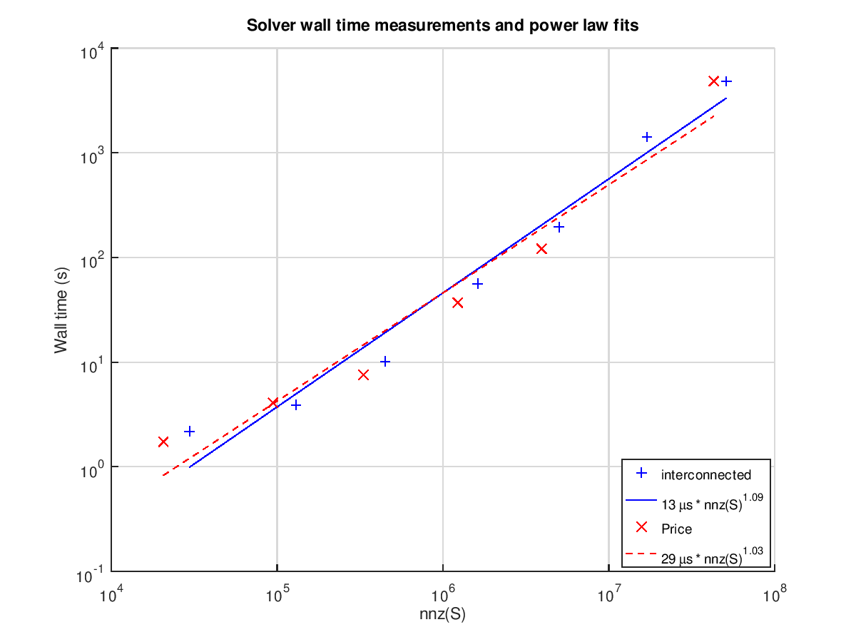
The nearly linear fit is very promising. Keep in mind that this is for this specific class of problems, and almost surely does not apply to solving LPs in general.

Some of the runs don't quite make it below the 1% mark:

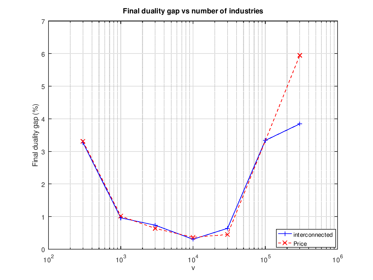
This suggests that there is more work to be done. A similarly shaped graph comes out when plotting the total number of conjugate gradient steps vs the number of industries:

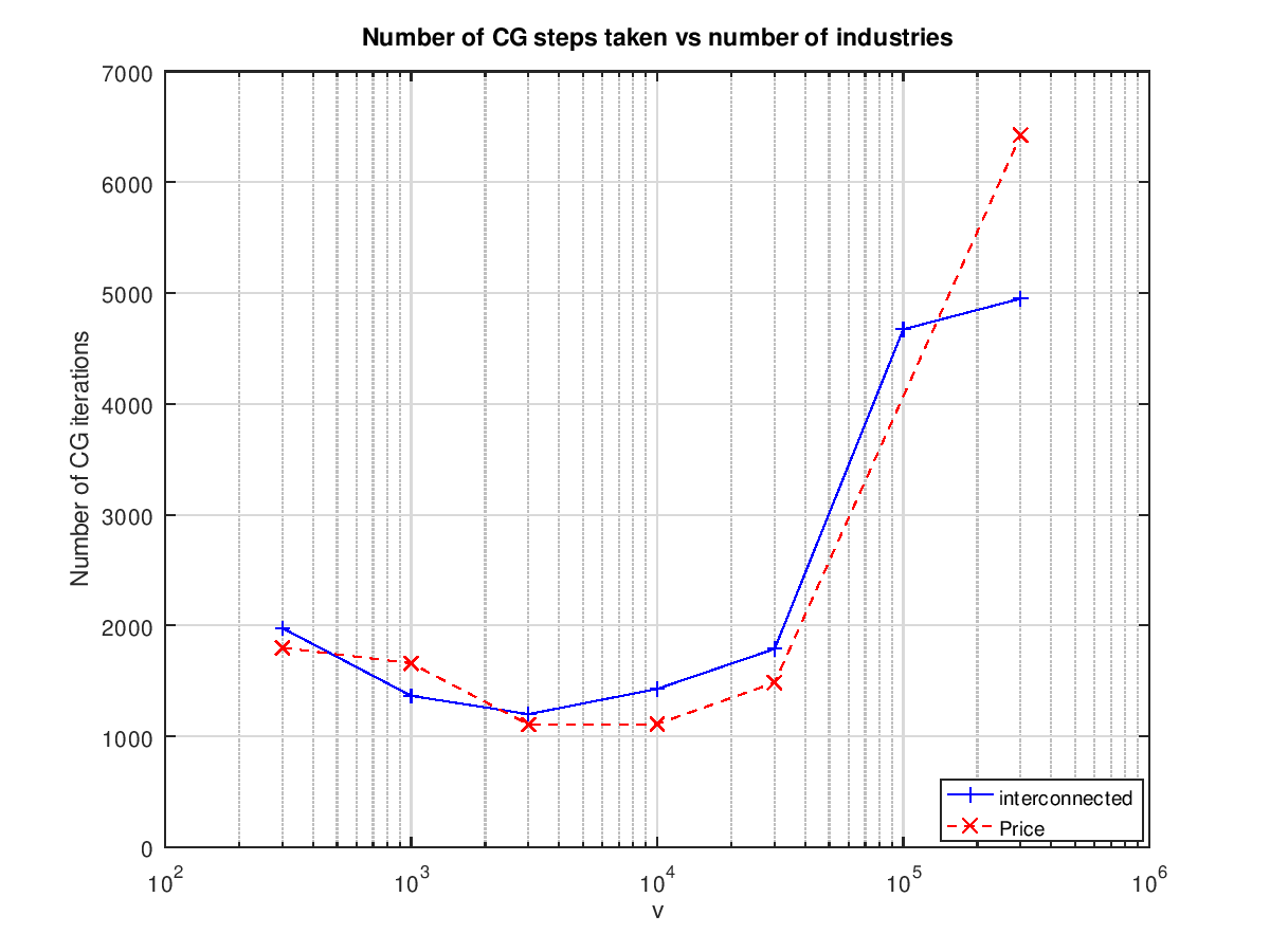
Interestingly the number of steps is between 1000 and 2000 for the runs that do find a 1% solution.

Parallelism

The central operation in Renegar's algorithm and its descendants is the centering Newton step. Recent work in the field has focused on speeding this up by maintaining an approximate inverse of the left-hand matrix. See for example the work of Lee and Sidford. These efforts are serial, and not as useful for dealing with sufficiently large systems.

Another way to deal with this is to parallelize the Newton solver. If we let the number of nodes scale with the number of non-zeroes in $S$ then the time for each step becomes constant, plus some communication overhead. If we use Renegar's more conservative result for the number of steps, then the total time to solve the LP is $O(\sqrt{m}L)$. From the experiment presented here we know that a single computer with 8 GiB of RAM can deal with a linear program corresponding to an economy with one million industries. It therefore does not seem unreasonable that the entirety of the world economy, a system with billions of industries, could be planned using a relatively modest computer cluster.